A Step-by-Step Guide to Compressing LLM Key-Value Caches with TurboQuant

Introduction

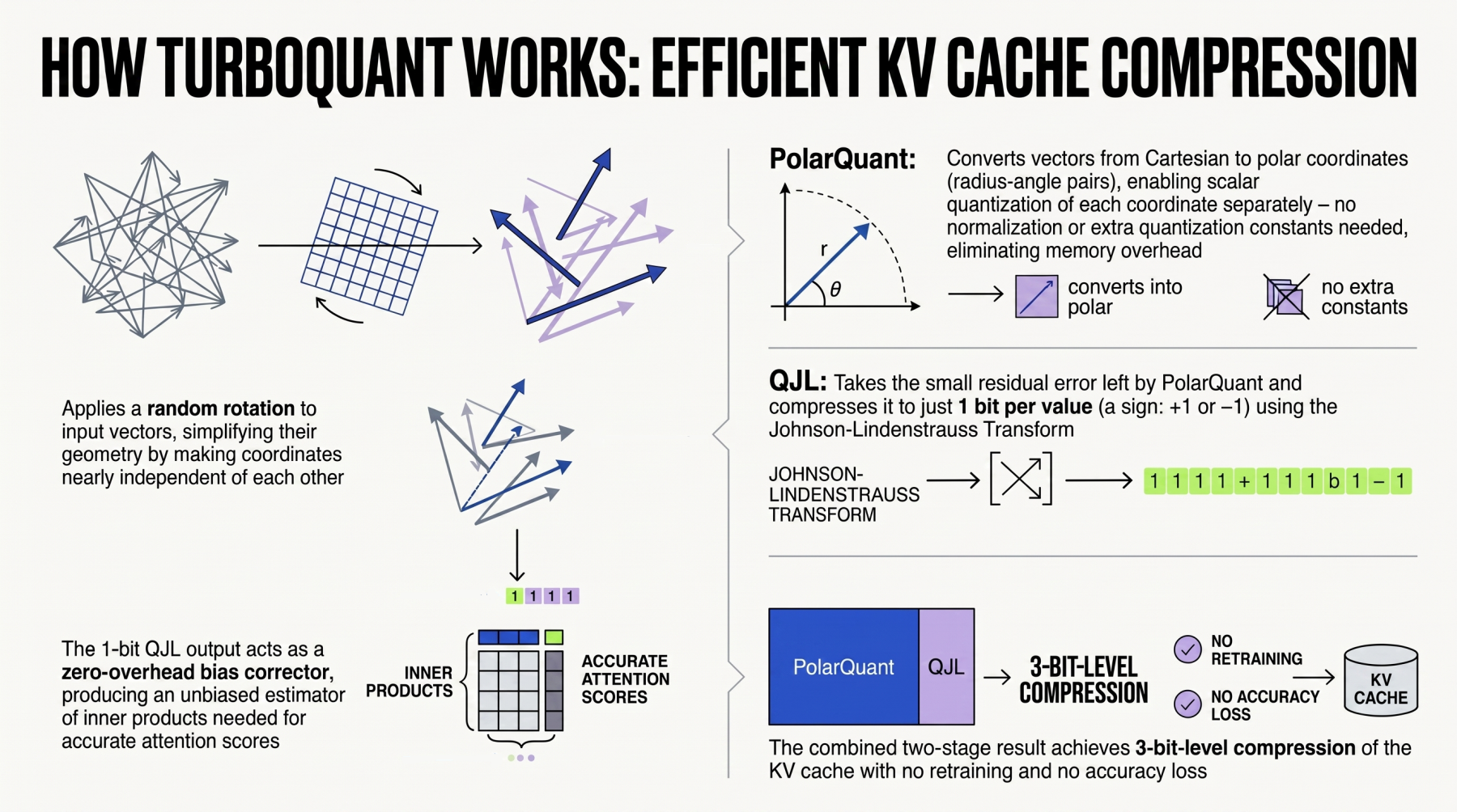
Large language models (LLMs) and retrieval-augmented generation (RAG) systems rely heavily on key-value (KV) caches to maintain context during inference. As model sizes grow, so do memory footprints, leading to increased latency and infrastructure costs. TurboQuant, recently launched by Google, offers a powerful algorithmic suite and library for applying advanced quantization and compression to LLMs and vector search engines. This guide walks you through the practical steps to compress KV caches using TurboQuant, enabling significant memory savings with minimal accuracy loss.

What You Need

• A pretrained large language model (e.g., GPT-style, LLaMA, or any transformer with KV cache)
• Python 3.8+ environment (virtual environment recommended)
• TurboQuant library (install via pip or from source)
• PyTorch or compatible deep learning framework (version >= 1.13)
• GPU with at least 8 GB VRAM for profiling and compression (optional but recommended)
• Basic understanding of quantization concepts (bit-width, scale, zero-point)

Step-by-Step Instructions

Step 1: Understand Your Model’s KV Cache Structure

Before applying compression, examine how your model stores and retrieves KV pairs. For transformer-based models, the KV cache is typically a dictionary of tensors keyed by layer index, containing keys and values from previous tokens. Use your framework’s model internals to inspect the cache shape, dtype, and number of layers. For example, in Hugging Face Transformers, you can access the cache via the past_key_values attribute after a forward pass. Note the tensors’ dimensions (batch, num_heads, seq_len, head_dim).

Step 2: Install TurboQuant

TurboQuant can be installed via pip:

pip install turboquant

Alternatively, clone the official repository from Google’s GitHub and install in editable mode for the latest features:

git clone https://github.com/google/turboquant.git
cd turboquant
pip install -e .

Verify the installation by running a simple test:

python -c "import turboquant; print(turboquant.__version__)"

This ensures all dependencies (like PyTorch, numpy, and custom CUDA kernels) are correctly set up.

Step 3: Profile the Memory Usage of the Original KV Cache

Before compression, establish a baseline. Run a few forward passes with your model using a representative input (e.g., a prompt of typical length). Use memory-profiling tools like torch.cuda.memory_summary() or NVIDIA Nsight to record the peak memory allocated to the KV cache. Also measure the inference latency per token. This baseline will help you evaluate the trade-offs of TurboQuant compression.

Step 4: Choose Quantization Parameters

TurboQuant supports several quantization schemes: uniform affine (8-bit, 4-bit) and non-uniform (e.g., normal float, quantile). The choice depends on your accuracy and memory budget. For KV caches, 8-bit uniform quantization often yields negligible accuracy loss while reducing memory by 4× (compared to FP32). To go further, 4-bit with per-channel quantization can achieve 8× compression, but requires careful calibration. Use TurboQuant’s built-in calibration tool to estimate the optimal bit-width and scale factors:

from turboquant.calibrate import calibrate_kv_cache
config = calibrate_kv_cache(model, calib_dataloader, target_compression=4.0)

This function analyzes the distribution of key and value tensors and suggests quantization parameters (e.g., bit_width=8, symmetric=True).

Step 5: Apply Quantization to the KV Cache

With configuration in hand, wrap your model’s KV cache logic with TurboQuant’s quantizer. The library provides a convenient QuantizedCache class that seamlessly replaces the standard cache during inference:

from turboquant.cache import QuantizedCache
qc = QuantizedCache(config)
outputs = model(input_ids, past_key_values=qc)  # qc handles quantization on the fly

For offline compression (e.g., pre-processing a cache for a fixed context), you can encode the KV tensors directly:

from turboquant.quantize import quantize_tensor
q_keys = quantize_tensor(keys, bit_width=4, symmetric=False)
q_values = quantize_tensor(values, bit_width=4, symmetric=False)

TurboQuant also supports mixed-precision caches, where earlier layers use higher bit-widths than later layers—useful when different layers have varying sensitivity to quantization.

Step 6: Validate Accuracy and Performance

After compression, run your model on a validation dataset (e.g., a subset of WikiText or your own QA prompts). Compare the perplexity, BLEU score, or downstream task accuracy before and after quantization. TurboQuant provides a validation module:

from turboquant.evaluate import evaluate_perplexity
orig_ppl = evaluate_perplexity(model, val_data, use_original_cache=True)
quant_ppl = evaluate_perplexity(model, val_data, use_quantized_cache=qc)
print(f"Original PPL: {orig_ppl:.2f}, Quantized PPL: {quant_ppl:.2f}")

Acceptable increase depends on your application—typically <1% degradation is considered safe. Also measure inference speed: the quantized cache may be slower if using low bit-widths due to dequantization overhead, but often the memory reduction allows larger batch sizes, improving throughput.

Step 7: Deploy the Compressed Model

Once validated, integrate the quantized cache into your production pipelines. TurboQuant supports exporting the quantization parameters as a lightweight JSON file, so you can reload them without recalibrating:

qc.save_config("turboquant_cache_config.json")
# Later: qc = QuantizedCache.load_config("turboquant_cache_config.json")

If you use a vector search engine (e.g., for RAG), TurboQuant can also compress the index embeddings using similar techniques. Follow the same workflow but replace QuantizedCache with QuantizedIndex provided by the library.

Tips for Best Results

• Start with 8-bit quantization—it’s often a sweet spot between memory savings and quality.
• Use a calibration dataset that closely matches your deployment queries to ensure the quantization ranges are optimal.
• Monitor the perplexity increase on a held-out set; if it exceeds 2%, try per-group quantization (e.g., per token or per head) to retain more precision.
• For RAG systems, compress the KV cache of the retriever separately from the generator—each may tolerate different quantization.
• Leverage TurboQuant’s KV cache fusion feature, which combines quantization with memory transfer optimizations to reduce CPU-GPU communication.
• Always benchmark end-to-end latency and memory, as quantized caches can reduce memory bandwidth bottlenecks.
• If your model uses positional embeddings in the KV cache, ensure those are excluded from quantization or handled with higher precision.

By following these steps, you can unlock the full potential of TurboQuant to shrink your LLM’s memory footprint while maintaining high-quality outputs—a critical step toward scalable and cost-effective AI systems.